yeungpinghei.github.io

An introduction to Generalised Additive Mixed Models (GAMMs)

Author: Ping Hei Yeung
Affiliation: Georgetown University
Published: May 11, 2023

What is GAMM?

Generalized Additive Mixed Models (GAMMs; Wood 2017) are an extension of Generalized Linear Mixed Models that allow for more flexible modeling of nonlinear relationships between the depdendent and independent variables. A relatively new approach, GAMMs have received increased attention in recent sociophonetic studies that involve the analysis of vowel formants (Kirkham et al., 2019; Stanley et al., 2021) and articulatory measurements (Carignan et al., 2020). GAMMs are comparable to linear mixed effect modeling, but they differ in how they model the relationships between depdendent and independent variables. In linear mixed effect modeling, the relationships between the variables are typically modeled using linear functions. In GAMMs on the other hand, the relationships between the variables are modeled using smooth functions, such as splines or smoothing splines. These smooth functions can capture more complex and nonlinear relationships between the variables, which allows for the modeling of nonlinear differences like vowel formant trajectories. Therefore, GAMMs have a major advantage in modeling dynamic acoustic and articulatory data like vowel formant trajectories and F0 contours which are nonlinear in nature.

In this tutorial, you will learn the basics of generalized additive mixed modelling (GAMM) using my data on Hong Kong English as an example. This tutorial is inspired by Wieling (2018) and modifications have been made to suit my own data.

Check out the tutorial by Winter & Wieling (2016), Sóskuthy (2017, 2021), and Wieling (2018) for more sophisticated explanations on the mechanisms of GAMMs.

Our sample data: tones in Hong Kong English

In this study, I want to find out if Hong Kong English is a tone language. According to recent studies on Hong Kong English like Wee (2016) and Gussenhoven (2014), monosyllabic content words may have a high tone while monosyllabic function words may have a low tone. I want to know if that is really the case, so I asked speakers of Hong Kong English and American English to read those words, and I extracted the F0 contours they produced using Praat. As you can see in Figure 1, speakers of Hong Kong English tend to produce content words like four with a higher pitch than function words like for.

Figure 1. The F0 contour of a Hong Kong English speaker saying Say four again and Say for again: HKE example Listen to it:

On the other hand, speakers of American English like the one in Figure 2 seem to produce both the content words and the function words with the same pitch. You may compare the two figures and see how they differ.

Figure 2: The F0 contour of a American English speaker saying Say four again and Say for again: AE example Listen to it:

However, just by looking at the raw F0 contour alone is not enough to answer my research question. How do I know if the difference between Hong Kong English and American English is statistically significant? In the next section, I will provide a step-by-step guide on how I used GAMM to analyze the data.

I will present my findings at ICPhS 2023 this August, so please come if you want to know more about my study! My paper is titled “Contact-induced tonogenesis in Hong Kong English” and it should be available soon on the conference website.

Step 0: A brief introduction of the data

First, download the R script gamm_tutorial.R and the csv file gamm_tutorial.csv from the Github repository.

Open the R script on RStudio and load the packages we need.

# Load the packages
library(tidyverse)
library(mgcv)
library(itsadug)
library(tidymv)

Import the csv file and define the data type of each column.

data <- read_csv("gamm_tutorial.csv", col_names = T)
data <- data %>%
  mutate_at(c("speaker", "variety", "gender", "word", "token", "cat","adjacent"), as.factor) %>%
  mutate_at(c("age", "duration", "repetition", "point", "F0", "semitone.norm"), as.numeric)
summary(data)

word	adjacent	speaker	variety	age	gender	duration	repetition	point	F0	token	semitone.norm	cat
an	null.son	AME_007	AE	19	F	0.429388633	3	8	200.8319991	AE_007-an-3	0.634121036	function
an	null.son	HKE_024	HKE	28	F	0.277847326	1	1	211.5430769	HKE_024-an-1	1.173468235	function
an	null.son	AME_013	AE	21	M	0.363250934	1	5	139.3838609	AE_013-an-1	-0.285611094	function
an	null.son	HKE_006	HKE	19	F	0.354345514	1	2	242.4686589	HKE_006-an-1	-0.003444452	function
an	null.son	HKE_012	HKE	24	M	0.164787882	2	4	97.84136779	HKE_012-an-2	-0.064295015	function
an	null.son	HKE_023	HKE	30	M	0.227550751	1	5	116.2275949	HKE_023-an-1	-0.517019108	function
an	null.son	AME_023	AE	20	F	0.390254703	1	6	201.8185885	AE_023-an-1	-0.289436547	function
an	null.son	HKE_010	HKE	38	F	0.247996446	1	9	140.0242878	HKE_010-an-1	-1.458272919	function
an	null.son	AME_033	AE	18	M	0.207696414	2	2	93.90499073	AE_033-an-2	-1.735087432	function
an	null.son	HKE_038	HKE	35	F	0.22003899	2	5	180.9764375	HKE_038-an-2	-0.992133573	function

In in csv file, each row represents an F0 measurement, with columns:

speaker: a unique code for each speaker
variety: the English variety spoken by the participant, American English (AE) or Hong Kong English (HKE)
age: age of the speaker
gender: gender of the speaker
word: the word from which the measurement was taken
duration: duration (in seconds) of the target word
repetition: each target word was repeated three times (1-3)
point: 9 equidistant F0 measurements were made at the 10%-90% intervals of the target words (1-9)
F0: the raw F0 measurements from Praat
token: the three columns speaker, word, and repetition combined into one
semitone.norm: the F0 measurements converted to semitones and z-score normalized by speaker
cat: the syntactic category of the target word, content word (content) or function word (function)
adjacent: the onset and coda consonants of the target word

Before applying any statistical models, we may first visualize the original data to check how they look like.

# Normalized F0 trajectory of each token by individual speakers
data %>%
  ggplot(aes(x = point, y = semitone.norm, color = cat, group = token)) + 
  geom_line() +
  facet_wrap(~speaker)

Many lines

Here we have the normalized F0 contours of each speaker, but it’s hard for us to pick up any patterns from the graph since the individual lines are messy.

Let’s make a geom_smooth() plot to see what speakers of Hong Kong English and American English did in general.

# Normalized F0 trajectory by syntactic category and English variety
data %>%
  group_by(speaker,cat,point,variety) %>%
  summarise(mean = mean(semitone.norm)) %>%
  ggplot(aes(x = point, y = mean, group = cat, color = cat)) +
  geom_smooth(method="loess") +
  facet_wrap(~variety)

geom_smooth

We can see that speakers of Hong Kong English and American English produced the content words and function words with differnt pitch contours. As indicated by the overlap of the 95% confidence interval (the shaded area), the pitch contour of content words and function words did not differ significantly for American English speakers. Speakers of Hong Kong English on the other hand produced the content words with a much higher F0 than the function words, and there was no overlap of the confidence intervals. However, this graph does not the consider the effect of other factors on pitch production like adjacent segments, number of repetion and duration, which may all contribute to the F0 difference. Thus, the effect of syntactic category on F0 may be overestimated.

Step 1: The most basic linear model

In this step, we construct a very basic linear regression model using the bam() function with the normalized F0 semitone.norm as the dependent variable and the syntactic category cat as the independent variable. Essentially, the model estimates the average difference in normalized F0 between function words and content words. The argument data refers to the data frame containing the dependent and independent variables, which is named as data in our case. The argument method specifies the estimation method we use for the smoothing parameter. Here we may use the default method "fREML", fast restricted maximum likelihood estimation. We will start from here and expand our model bit by bit.

m1 <- bam(semitone.norm ~ cat, data=data, method="fREML")

To obtain a summary of the model, we can use the summary() function.

summary(m1)

m1_summary

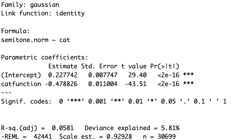
First part of the model summary:

The family of model used (Gaussian model), the link function (identity) and the model formula.

Parametric coefficients:

The intercept is the value of the dependent variable when all numerical predictors are equal to 0 and nominal variables are at their reference level. Since the reference level for the nominal variable cat is ‘content’, the average normalized F0 of content words is about 0.23.
The line associated with catfunction (function word, the non-reference level) indicates that the normalized F0 of function words is about 0.48 lower than that of content words, and this difference is significant with a very small p-value (p<2e-16).

The final two lines of the summary show the goodness-of-fit statistics.

R-sq.(adj) represents the amount of variance explained by the regression.
Deviance explained is a generalization of R-sq.
REML (restricted maximum likelihood) by itself is not informative. Its value is only meaningful when two models are compared which are fit to the same data, but only differ in their random effects. A lower value means that the model is a better fit to the data. For models with non-linear patterns, the REML label is replaced by fREML.
Scale est. represents the variance of the residuals.
n is the number of data points in the model.

Step 2: Include a smooth for change in F0 over time

Then, how can we account for the the changes in F0 over the time in our model? GAMM allows us to assess non-linear patterns by using smooths, which model nonlinear patterns by combining a pre-specified number of basis functions. To include a nonlinear pattern over time, our model can be specified as follows:

m2 <- bam(semitone.norm ~ cat + s(point, by=cat,bs="tp", k=9), data=data)
summary(m2)

Compared to m1, the first model, we added the function s(point, by=cat,bs="tp", k=9), a smooth over point, the time point which the measurement was taken. The argument by=cat means that the smooths were made separately for each level of the nominal variable of syntactic category. The bs parameter specifies the type of smooth, and in this case is set to “tp”, the default thin plate regression spline. The k parameter sets the size of the basis dimension. The value of k cannot exceed the number of possible values of the smooth term. Therefore, we set it to 9 as there are only 9 possible values of point (F0 was measured at 9 points in time for each token).

m2_summary

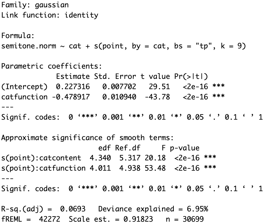
The summary of the new model has an additional block, the approximate significance of smooth terms. Here two lines can be found, s(point):catcontent, the smooth for content words and s(point):catfunction, the smooth for function words. The p-value associated with each smooth indicates if the smooth is significantly different from 0. Since both smooths have the p-value of <2e-16 , they are significantly different from 0.

Ref.df is the reference number of degrees of freedom used for hypothesis testing (on the basis of the associated F-value). edf is the number of effective degrees of freedom, which can be seen as an estimate of how many parameters are needed to represent the smooth. It is also indicative of the amount of non-linearity of the smooth. The higher the edf value, the more complex (i.e. non-linear) the smooth. The maximum value of edf is k minus one, so it would be 8 in our case. If the edf value is close to its maximum, then a higher basis dimension might be necessary to prevent oversmoothing. The values we have are 5.317 and 4.938, which are not close to the maximum of 8. It means that the k value we chose is suitable for our model.

We may visualize the results of GAMM using plot_smooth() and plot_diff() from the itsadug package. Visualization is essential since the model summary may not give you the full picture on the effects of the independent variable. While it is possible to summarize a linear pattern in only a single line, this is obviously not possible for a non-linear pattern like F0 trajectory. The function words and content words may significantly differ in their F0 only in part of the word but not the whole word, but model summaries are not able to distinguish that. Instead, by plotting the results of GAMMs, we may find out the exact time intervals with significant difference.

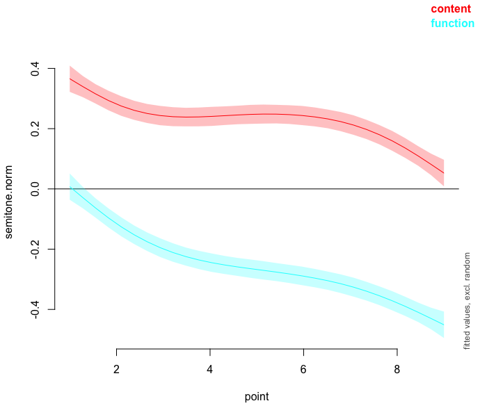
plot_smooth(m2, view="point", plot_all= "cat", rug=FALSE)
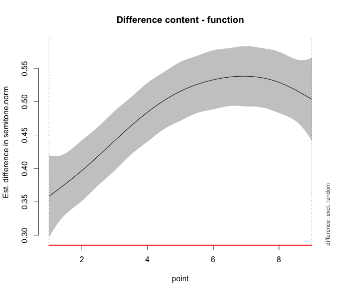
plot_diff(m2, view="point", comp=list(cat=c("content","function")))

The first parameter is the name of the model, which is m2 in this case. The second paramter view is set to the variable we want to visualize, which is ‘point’. The parameter plot_all, which is only present in plot_smooth(), is set to the nominal variable of syntactic category cat. The parameter comp, which is only present in plot_diff() specifies the list of the variables what are compared. For this plot, we want to compare content words content and function words function from the variable of cat. The final parameter rug serves to show or suppress small vertical lines on the x-axis for all individual data points. This plotting function only visualizes the partial effects of the two non-linear patterns since the other components of the model are not incorporated.

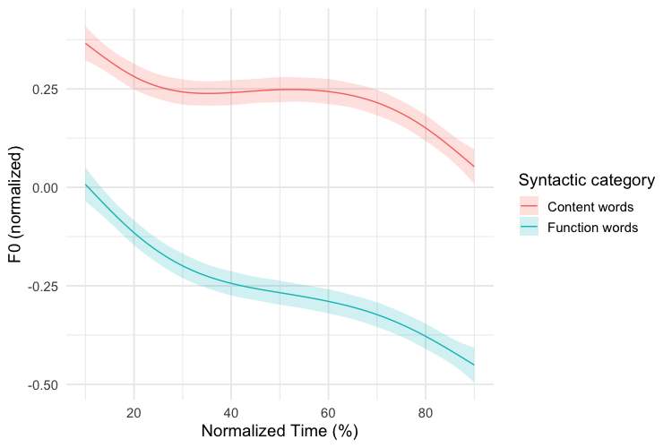
The graph on the left shows the output of plot_smooth(), which indicates the non-linear smooths for function words and content words of the model m2. In other words, these are the predicted F0 trajectories of function words and content words according to the model. The 95% confidence intervals are shown by shaded bands.

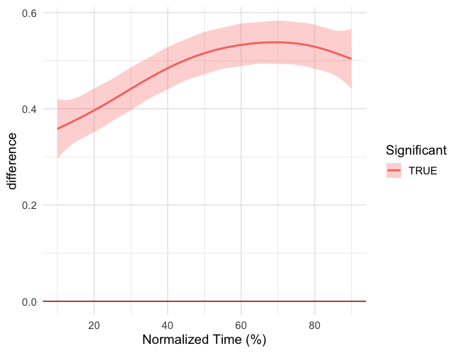
Then, the graph on the right shows the output of plot_diff, which is the difference between the two non-linear smooths of the model m2 comparing function words and content words. The 95% confidence interval is shown by a shaded band. If the confidence interval does not overlap with the x-axis, then the difference is significant. As shown in the plot, there is no overlap of the confidence interval, indicating that content words have a significantly higher normalized F0 than function words throughout the entire duration of the words.

You may also plot the results using ggplot(), which gives you more freedom to customize the plots. You may follow the tutorial by Dr. Stefano Coretta to learn more about how to visualize the results of GAMMs using ggplot().

The code for plotting the model predictions:

m2 %>%
  get_gam_predictions(point, series_length = 150, exclude_random = TRUE) -> m2.predictions
m2.predictions %>%
  ggplot(aes(point * 10, semitone.norm)) +
  geom_ribbon(aes(ymin = CI_lower, ymax = CI_upper, fill = cat, group = cat), alpha = 0.2) +
  geom_line(aes(colour = cat)) +
  scale_x_continuous(name = "Normalized Time (%)", breaks = seq(0, 100, by=20)) + 
  scale_y_continuous(name = "F0 (normalized)") +
  scale_color_discrete(name = "Syntactic category", labels = c("Content words","Function words")) +
  scale_fill_discrete(name = "Syntactic category", labels = c("Content words","Function words")) +
  theme_minimal(base_size = 14)

m2.predictions

The code for plotting the difference smooth:

m2 %>%
  get_smooths_difference(point, list(cat = c("content", "function"))) -> m2.diff
m2.diff %>%
  ggplot(aes(point*10, difference, group = group)) +
  geom_hline(aes(yintercept = 0), colour = "darkred") +
  geom_ribbon(aes(ymin = CI_lower, ymax = CI_upper, fill = sig_diff), alpha = 0.3) +
  geom_line(aes(colour = sig_diff), size = 1) +
  scale_x_continuous(name = "Normalized Time (%)", breaks = seq(0, 100, by=20)) +
  labs(colour = "Significant", fill = "Significant") +
  theme_minimal(base_size = 14)

m2.diff

Step 3: Include random intercepts for speakers and words

Then, we want to account for the random effects of individual speakers and words. To do so, we may add the random-effect smooths of s(speaker,bs="re") and s(word, bs="re"). The first parameter is the random-effect factor, which is interpreted as a random intercept.

m3 <- bam(semitone.norm ~ cat +
                s(point, by=cat, k=9) +
                s(speaker,bs="re") +
                s(word, bs="re"),
              data=data)
summary(m3)

m3_summary

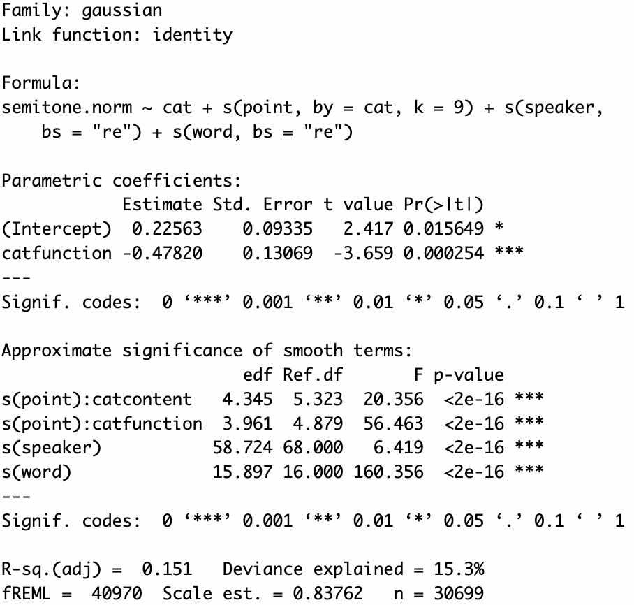
The p-values of s(speaker) and s(word) in the model summary tell us whether the random intercepts are necessary. In this case, since the p-values are both significant (p<2e-16), we should keep these two random intercepts.

To figure out whether we should include the random intercepts, we may also compare models with and without them using the compareML() function from the itsadug package. It uses the Akaike Information Criterion (AIC) to compare the goodness of fit of the two models while taking into account the complexity of the models. To use this function, the models must have the same fixed effects. Or else, the maximum likelihood (ML) estimation method should be used instead. Therefore, in order to compare m2 and m3, we have to refit them using ML.

m2.ml <- bam(semitone.norm ~ cat + s(point, by=cat,bs="tp", k=9), data=data, method="ML")
m3.ml <- bam(semitone.norm ~ cat + s(point, by=cat, k=9) + s(speaker,bs="re") + s(word, bs="re"), data=data, method="ML")

Then, we can compre the models:

# Model comparison
compareML(m2.ml,m3.ml)

compare

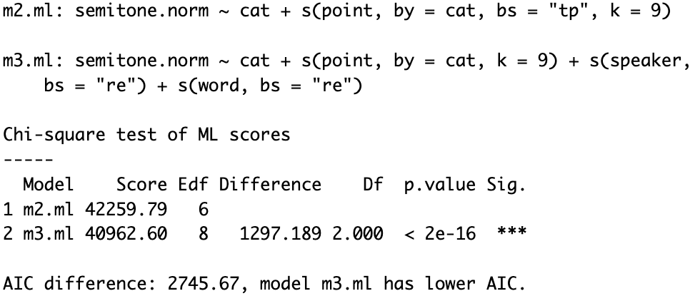
The results show that the model m3.ml is better since it has a lower AIC score. Therefore, it is better for us to include the random intercepts.

Step 4: Include by-speaker random slopes

Question: What is the difference between random intercepts and random slopes?

Some speakers or words will on average have a higher F0 than others, and this structural variability is captured by a by-speaker or by-word random intercepts. On the other hand, the exact difference in F0 between content and function words may vary per speaker. Random slopes allow the influence of a predictor to vary for each level of the random-effect factor.

To include a by-speaker linear random slope for the effect of syntactic category, we can replace s(speaker,bs="re") with s(speaker, cat, bs="re") to our model. It is not recommended to include both smooths in the model since that would be redundant.

m4 <- bam(semitone.norm ~ cat +
                s(point, by=cat, k=9) +
                s(word, bs="re") +
                s(speaker, cat, bs="re"),
              data=data)
summary(m4)

m4_summary

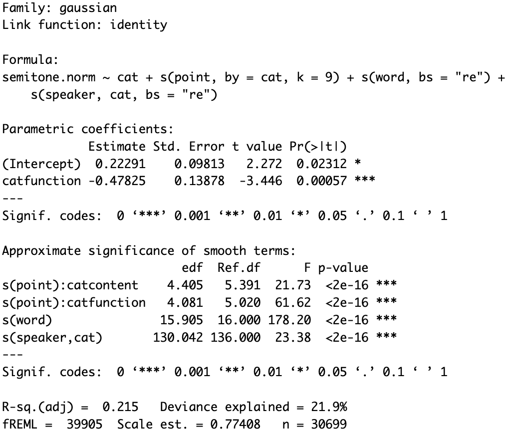
The model summary shows a significant effect of s(speaker, cat), supporting the inclusion of the random slope.

Step 5: Include non-linear random effects

Although we have added random intercepts and random slopes to our model, we still haven’t accounted for the non-linear random effects of speakers on normalized F0 over time. Thus, we should replace the random slope s(speaker, cat, bs="re") with the smooth specification s(point, speaker, by=cat, bs="fs",m=1), which allows us to model the variable effect of syntactic category on individual speakers over time. The random intercept for speakers is dropped because the difference is incorporated by the non-centered factor smooth. The first parameter point represents the non-linear difference over time while the second parameter speaker refers to the general time pattern for each individual speakers. by=cat allows for individual variability in the effect of syntactic category. The parameter bs is now set to “fs”, indicating that it is a factor smooth. The final parameter, m, indicates the order of the non-linearity penalty.

Note: The code may take some time to run since the model is getting more complex.

m5 <- bam(semitone.norm ~ cat +
                s(word, bs="re") +
                s(point, speaker, by=cat, bs="fs", m=1),
              data=data)
summary(m5)

m5_summary

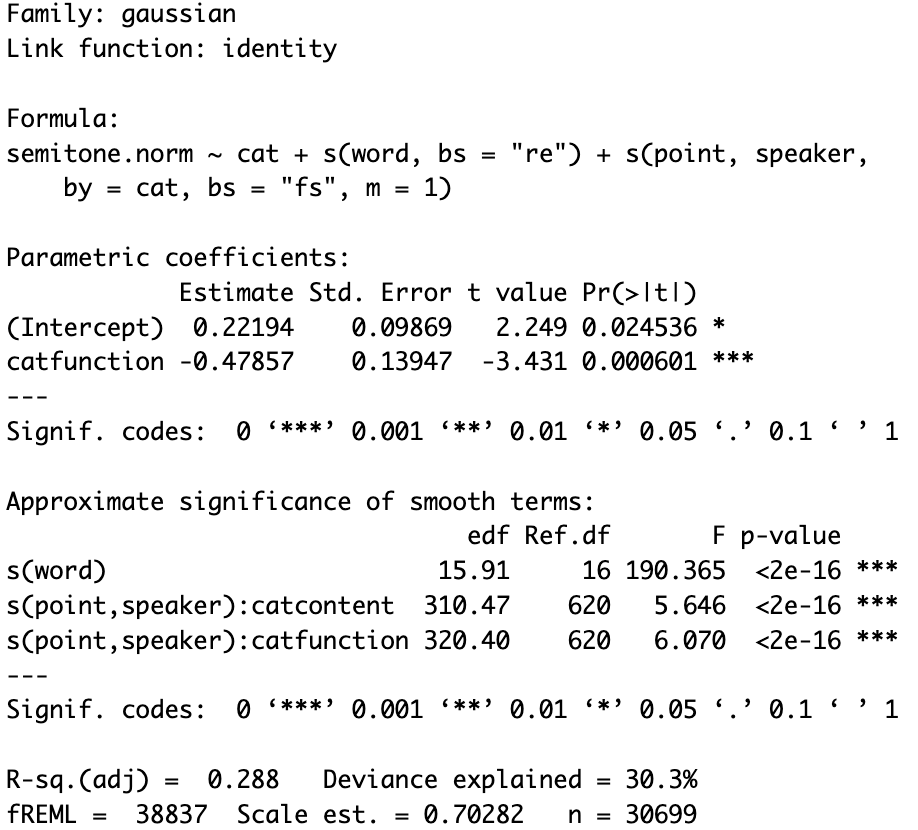
According to the model summary, both factor smooths ’s(point, speaker):catcontent’ and ’s(point, speaker):catcontent’ have a significant p-value of <2e-16. Thus, it is necessary to include them in our model.

Step 6: Account for autocorrelation in the residuals

As we are analyzing time-series data, we should be aware of autocorrelation in the residuals. It refers to the degree to which the differences between the actual values and the predicted values in a time series are correlated with one another over time. Specifically, autocorrelation occurs when the residuals at one point in time are correlated with the residuals at another point in time. Using the acf_resid function from the itsadug package, we can generate a autocorrelation graph to check the degree of autocorrelation in our model.

m5.acf <- acf_resid(m5)

acf_resid

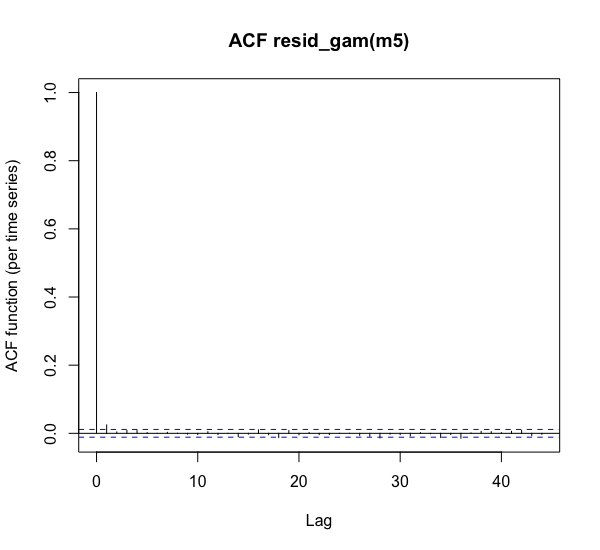
The first vertical line in the graph is always at height 1, meaning that each point has a correlation of 1 with itself. The second line shows the amount of autocorrelation present when comparing measurements at time t-1 and time t. The value is very low at around 0 in this model, meaning that each additional time point yields a lot of additional information. However, if the amount of autocorrelation is high, we should incorporate an AR(1) error model for the residuals. It is important to note that autocorrelation can only be assessed adequately if the dataset is ordered. Hence, for each individual token (speaker + word + repetition), the rows have to be ordered by increasing time. Each separate time series in the dataset should be positioned one after another. To do so, we may use the function below to create a new column in the dataset that indicates whether an F0 measurement is the first one within the token.

data <- data %>%
  arrange(speaker, word, repetition, point) %>%
  group_by(speaker, word, repetition) %>%
  mutate(start.event = case_when(point == min(point) ~ TRUE, TRUE ~ FALSE), .after = point)

Then, we can incorporate an AR(1) error model for the residuals into our model specification with rho=m5.acf[2], AR.start=data$start.event. The first parameter added is rho, which is an estimate of the amount of autocorrelation. Using the height of the second line in the autocorrelation graph [2] is generally a good estimate. The second parameter added is AR.start, which should be the new column we just created in the dataset.

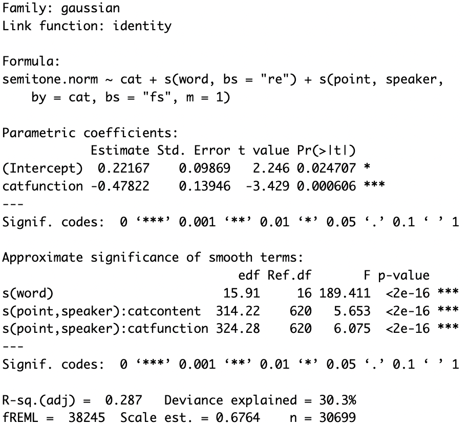
m6 <- bam(semitone.norm ~ cat +
                s(word, bs="re") +
                s(point, speaker, by=cat, bs="fs", m=1),
              data=data,
              rho=m5.acf[2], AR.start=data$start.event)
summary(m6)

m6_summary

Step 7: Include two-dimensional interaction

Using two-dimensional non-linear interactions, we can incorporate interactions that involve two numerical predictors like the one between time and repetition. Since the predictors point and repetition are not on the same scale (there are 9 possible values of point but 3 possible values of repetition), a tensor product smooth interaction should be used. A tensor product models a non-linear interaction by allowing the coefficients underlying the smooth for one variable to vary non-linearly depending on the value of the other variable. Using the te function, a tensor product te(point, repetition, k=3) can be included in our model specification. By default, the te-constructor uses two 5-dimensional cubic regression splines (bs=”cr”) and hence the k-parameter is set to 5. However, since there are only 3 possible values of repetition, we would set k to 3 instead.

m7 <- bam(semitone.norm ~ cat +
                te(point, repetition, k=3) +
                s(word, bs="re") +
                s(point, speaker, by=cat, bs="fs", m=1),
              data=data)
summary(m7)

m7_summary

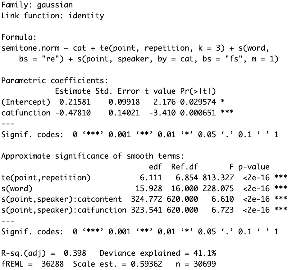
According to the model summary, the two-dimensional interaction between time and repetition ‘te(point, repetition)’ has a significant p-value of <2e-16. Thus, it is beneficial to include it in our model.

Step 8: Compare Hong Kong English and American English

So far we have considered the effect of syntactic category on normalized F0, but we have yet to explore if it affects speakers of Hong Kong English and American English equally. One may be tempted to construct two separate models for Hong Kong English and American English, but it is not an ideal appraoch. If we fit two separate models, we would not be able to evaluate whether the addition of English variety is warranted. While a visual comparison may give us the impression that the two patterns are different, the difference between them may not be significantly different. Using the interaction() function, we may create new a column in the data frame, an interaction between syntactic category and English variety.

# Combine the two variables
data$cat.variety <- interaction(data$cat, data$variety)

Then, we can make it the independent variable instead of cat. We can also add a new factor smooth s(point, word, by=variety, bs="fs", m=1), which models variety-specific differences in the articulation of individual words.

# It takes a while to load...
m8 <- bam(semitone.norm ~ cat.variety +
            te(point, repetition, k=3) +
            s(point, speaker, by=cat, bs="fs", m=1) +
            s(point, word, by=variety, bs="fs", m=1),
          data=data)
summary(m8)

m8_summary

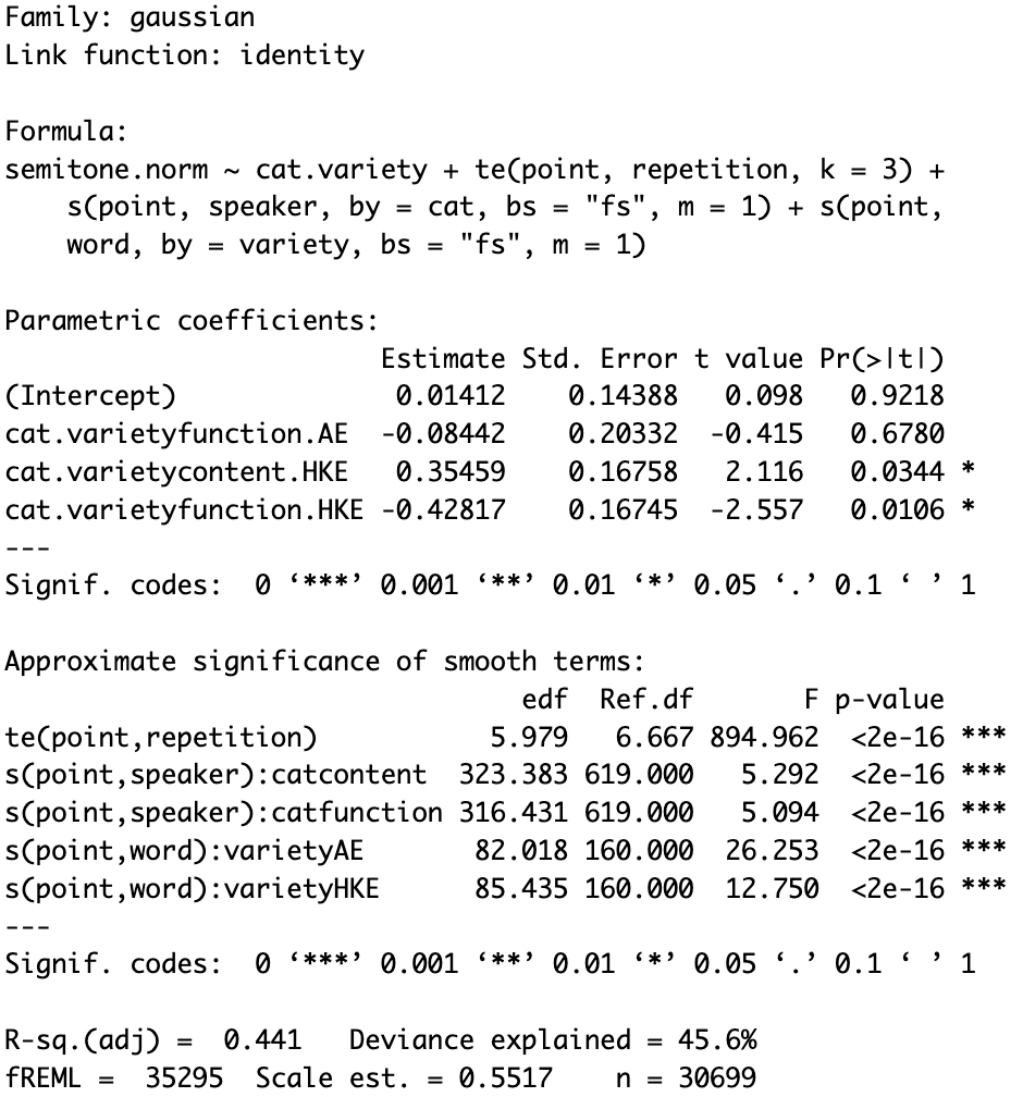
With content words produced by American English speakers as the baseline, the model summary shows that speakers of Hong Kong English had a significantly higher F0 for content words (p=0.0344) and a significantly lower F0 for function words (p=0.0106), while speakers of American English did not produce significant differences in F0 for these two syntactic categories (p=0.6780).

Step 9: Final model

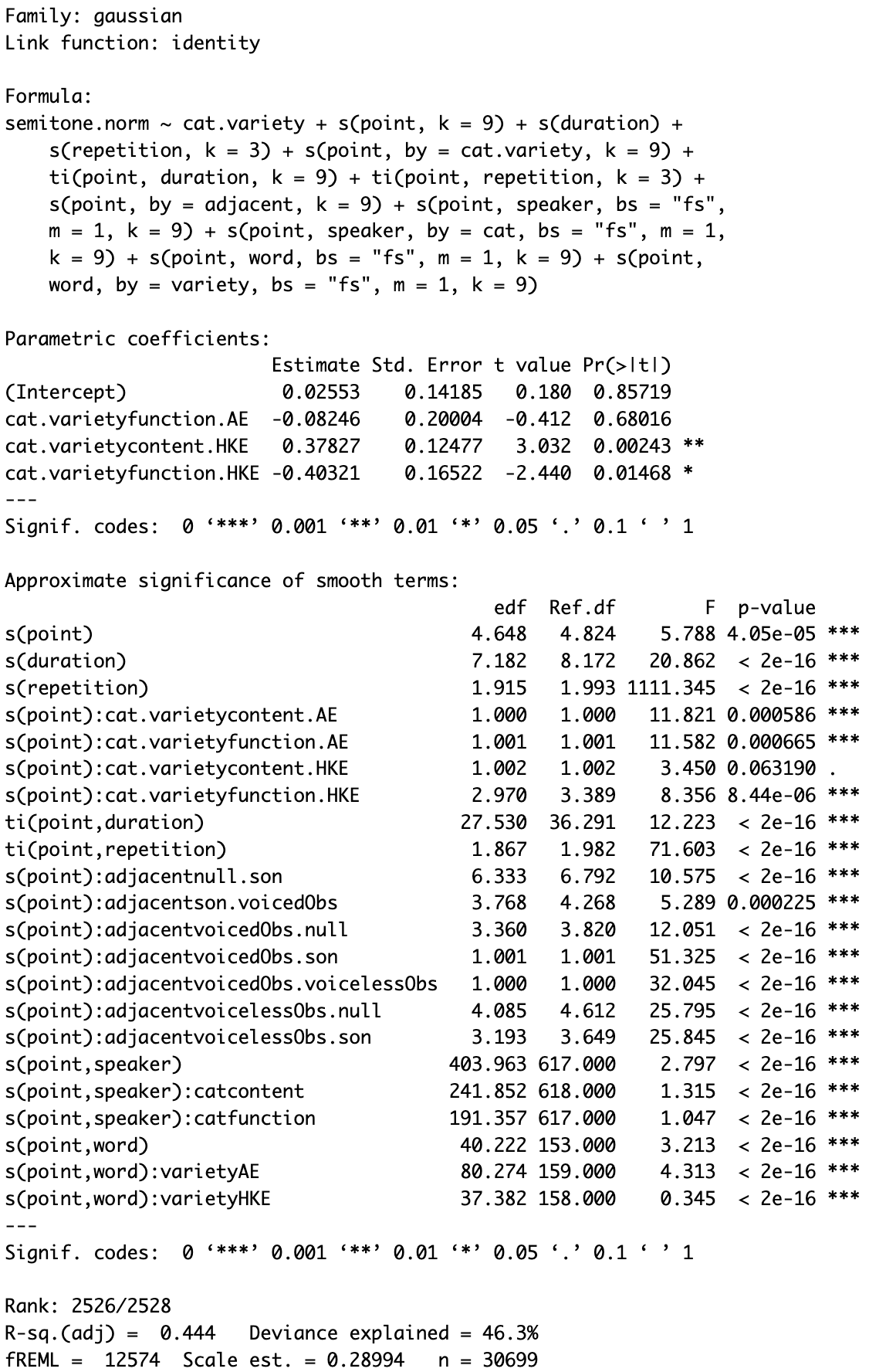
Here is the full model I created for my data. It includes all the fixed effects and random effects that are required.

m.full.noar <- bam(semitone.norm ~ cat.variety +
                     s(point, k=9) +
                     s(duration) +
                     s(repetition, k=3) +
                     s(point, by = cat.variety, k=9) +
                     ti(point, duration, k=9) + # Fixed interaction of duration x time
                     ti(point, repetition, k=3) + # Fixed interaction of repetition x time            
                     s(point, by = adjacent, k=9) + # Difference smooth for syllable structure
                     # Random Reference/Difference smooths for Speaker/Word
                     s(point, speaker, bs = 'fs', m = 1, k=9) +
                     s(point, speaker, by = cat, bs = 'fs', m = 1, k=9) +
                     s(point, word, bs = 'fs', m = 1, k=9) +
                     s(point, word, by = variety, bs = 'fs', m = 1, k=9),
                   discrete = TRUE, nthreads = parallel::detectCores(logical = FALSE) - 1,
                   data = data)
summary(m.full.noar)

The dependent variable was the normalized F0 semitone.norm. The independent variable was the interaction of English variety and syntactic category cat.variety. The reference level of this interaction term was content word by American English speakers. The interaction was included as a parametric effect and as a smooth s(point, by = cat.variety, k=9) in the model. The smooth included time point to indicate the normalized time point of the measurements. The smoothing term s(point, k=9) models the non-linear F0 values over time. The parametric effects of duration s(duration) and repetition s(repetition, k=3), as well as their fixed interactions with time ti(point, duration, k=9) and ti(point, repetition, k=3) were included to model their influence on F0. The difference smooth s(point, by = adjacent, k=9) accounted for the non-linear effect of adjacent segments. Random effect structure was also included in the model. speaker was included as a random intercept and slope interacting with cat to model the variable effect of syntactic category on individual speakers. word was included as a random intercept and slope interacting with variety to model variety-specific differences in the articulation of individual words.

Since the model is very complex, we need to find ways to speed up the calculation. It can be done by using discrete and nthreads. discrete reduces computation time by taking advantage of the fact that numerical predictors often only have a modest number of unique (rounded) values. nthreads speeds up the computation by using multiple processors in parallel to obtain the model fit.

m.full.acf <- acf_resid(m.full.noar)
m.full <- bam(semitone.norm ~ cat.variety +
                s(point, k=9) +
                s(duration) +
                s(repetition, k=3) +
                s(point, by = cat.variety, k=9) +
                ti(point, duration, k=9) +
                ti(point, repetition, k=3) +                
                s(point, by = adjacent, k=9) +
                s(point, speaker, bs = 'fs', m = 1, k=9) +
                s(point, speaker, by = cat, bs = 'fs', m = 1, k=9) +
                s(point, word, bs = 'fs', m = 1, k=9) +
                s(point, word, by = variety, bs = 'fs', m = 1, k=9),
              rho = m.full.acf[2], AR.start = data$start.event,
              discrete = TRUE, nthreads = parallel::detectCores(logical = FALSE) - 1,
              data = data
summary(m.full)

To account for the relationship between measurements taken at consecutive time points, an autoregressive error term was included. An AR1 model was incorporated to account for autocorrelation of residuals. The model was calculated using a scaled-t distribution to correct for non-normality of the model residuals.

You may save the full model to your computer using the saveRDS() function so that you don’t have to wait every time you run the script. The model output will be saved as an .rds file.

# Save the full model because we don't want to wait every time we run the script
saveRDS(m.full, file = "gamm_result.rds")

To import the GAMM output that you saved to RStudio, use the readRDS() function.

# Load the saved GAMM results to save your time
m.full <- readRDS("gamm_result.rds")

m9_summary

Step 10: Visualize the output of the final GAMM

Here I used the same codes as in Step 2 to visualize the output of my final GAMM.

m.full.predictions <- m.full %>%
  get_predictions(cond = list(cat.variety = c("content.AE","function.AE","content.HKE","function.HKE"), point=seq(1,9,0.1))) %>%
  mutate(lower = fit - CI, upper = fit + CI)
m.full.predictions <- separate(m.full.predictions, cat.variety, c("cat","variety"))
m.full.predictions %>%
  ggplot(aes(point * 10, fit)) +
  geom_ribbon(aes(ymin = lower, ymax = upper, fill = cat, group = cat), alpha = 0.2) +
  geom_line(aes(colour = cat)) +
  scale_x_continuous(name = "Normalized Time (%)", breaks = seq(0, 100, by=20)) + 
  scale_y_continuous(name = "Predicted F0 (z-score)") +
  scale_color_discrete(name = "Syntactic category", breaks = c("content","function"), labels = c("Content word","Function word")) +
  scale_fill_discrete(name = "Syntactic category", breaks = c("content","function"), labels = c("Content word","Function word")) +
  theme_minimal(base_size = 18) +
  facet_wrap(~variety)

gamm_result

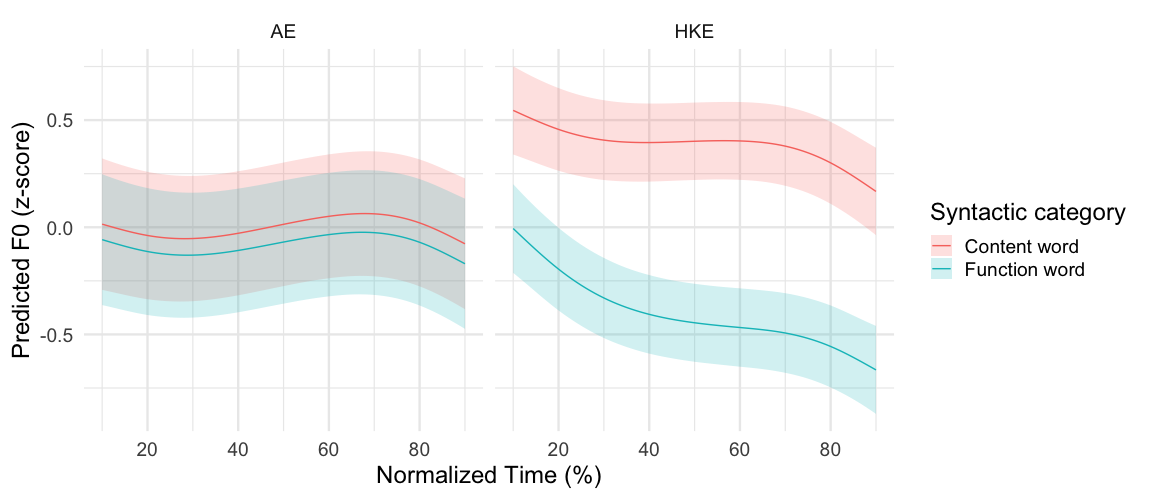
This figure provides the predicted F0 trajectory by each syntactic category for speakers of American English and Hong Kong English. Hong Kong English speakers produced the content words with a significantly higher F0 throughout the entire sonorant duration than the function words. For them, the 95% confidence interval of the content words did not overlap with that of the function words. Conversely, no clear patterns of pitch contour were observed for the American English group as the F0 stayed relatively constant throughout the sonorant duration regardless of syntactic category. There is a complete overlap of the 95% confidence intervals of the predicted F0 contours of content words and function words.

m.full %>%
  get_smooths_difference(point, list(cat.variety = c("function.HKE","content.HKE"))) -> hke.diff
hke.diff <- hke.diff %>%
  mutate(cat="function word - content word")
m.full %>%
  get_smooths_difference(point, list(cat.variety = c("function.AE","content.AE"))) -> ame.diff
ame.diff <- ame.diff %>%
  mutate(cat="function word - content word",variety = "AE")
diff <- rbind(hke.diff,ame.diff)
diff$variety = factor(diff$variety, levels=c('AE','HKE'))
diff %>%
  ggplot(aes(point*10, difference, group = group)) +
  geom_hline(aes(yintercept = 0), colour = "darkred") +
  geom_ribbon(aes(ymin = CI_lower, ymax = CI_upper, fill = sig_diff), alpha = 0.3) +
  geom_line(aes(colour = sig_diff), size = 1) +
  scale_x_continuous(name = "Normalized Time (%)", breaks = seq(0, 100, by=20)) +
  scale_y_continuous(name = "Predicted F0 difference (z-score)") +
  scale_color_discrete(breaks = c("TRUE","FALSE"), labels = c("Significant","Insignificant")) +
  scale_fill_discrete(breaks = c("TRUE","FALSE"), labels = c("Significant","Insignificant")) +
  labs(colour = "", fill = "") +
  theme_minimal(base_size = 18) +
  facet_grid(cat~variety)

gamm_diff

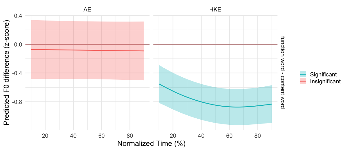
This figure on the other hand demonstrates the significance of the difference in F0 between the two syntactic categories for each variety. It also indicates a significant difference in F0 throughout the whole sonorant duration for Hong Kong English but not American English. Furthermore, the confidence intervals for each syntactic category in the American English group were wider than those of the Hong Kong English group, which indicates that American English speakers produced the target words with greater variability in F0.

In sum, the results of GAMMs indicate that speakers of Hong Kong English and American English differed in their F0 production of monosyllabic content and function words. Throughout the sonorant duration, Hong Kong English speakers produced the content words with a significantly higher F0 than function words, while no effect of syntactic category was found for American English speakers.

References

Carignan, C., Hoole, P., Kunay, E., Pouplier, M., Joseph, A., Voit, D., Frahm, J., & Harrington, J. (2020). Analyzing speech in both time and space: Generalized additive mixed models can uncover systematic patterns of variation in vocal tract shape in real-time MRI. Laboratory Phonology: Journal of the Association for Laboratory Phonology, 11(1), 2. https://doi.org/10.5334/labphon.214

Gussenhoven, C. (2014). On the intonation of tonal varieties of English. In M. Filppula, J. Klemola, & D. Sharma (Eds.), The Oxford Handbook of World Englishes. Oxford University Press.

Kirkham, S., Nance, C., Littlewood, B., Lightfoot, K., & Groarke, E. (2019). Dialect variation in formant dynamics: The acoustics of lateral and vowel sequences in Manchester and Liverpool English. The Journal of the Acoustical Society of America, 145(2), 784–794. https://doi.org/10.1121/1.5089886

Sóskuthy, M. (2017). Generalised additive mixed models for dynamic analysis in linguistics: A practical introduction (arXiv:1703.05339). arXiv. https://doi.org/10.48550/arXiv.1703.05339

Sóskuthy, M. (2021). Evaluating generalised additive mixed modelling strategies for dynamic speech analysis. Journal of Phonetics, 84, 101017. https://doi.org/10.1016/j.wocn.2020.101017

Stanley, J. A., Renwick, M. E. L., Kuiper, K. I., & Olsen, R. M. (2021). Back Vowel Dynamics and Distinctions in Southern American English. Journal of English Linguistics, 49(4), 389–418. https://doi.org/10.1177/00754242211043163

Wee, L. H. (2016). Tone assignment in Hong Kong English. Language, 92, e67–e87. https://doi.org/10.1353/lan.2016.0039

Wieling, M. (2018). Analyzing dynamic phonetic data using generalized additive mixed modeling: A tutorial focusing on articulatory differences between L1 and L2 speakers of English. Journal of Phonetics, 70, 86–116. https://doi.org/10.1016/j.wocn.2018.03.002

Winter, B., & Wieling, M. (2016). How to analyze linguistic change using mixed models, Growth Curve Analysis and Generalized Additive Modeling. Journal of Language Evolution, 1(1), 7–18. https://doi.org/10.1093/jole/lzv003

Wood, S. N. (2017). Generalized Additive Models: An Introduction with R, Second Edition (2nd ed.). Chapman and Hall/CRC. https://doi.org/10.1201/9781315370279